Altimetry diagnostics
This section show comparisons on geostrophic velocities computed from Sea Level Anomaly (SLA)
From Croco model, the SLA is computed from the difference between SSH and SSH integrated over the year.
\[SLA(t)=zeta(t)-zeta_{mean}\]Then the EKE is computed from geostrophic velocities
\[\begin{split}EKE=\frac{1}{2}*(u^{'2}+v^{'2}) \\ =\frac{g^2}{2f^2}*((\frac{-\partial{SLA}}{\partial{y}})^2+(\frac{\partial{SLA}}{\partial{x}})^2)\end{split}\]The Altimetry products used here are AVISO products which provide directly the components of geostrophic velocities ugosa and vgosa
https://www.aviso.altimetry.fr/en/data/product-information/aviso-user-handbooks.html
Filtering of Data
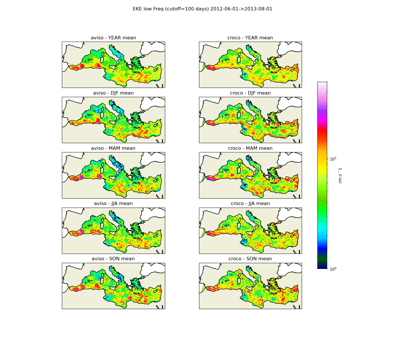
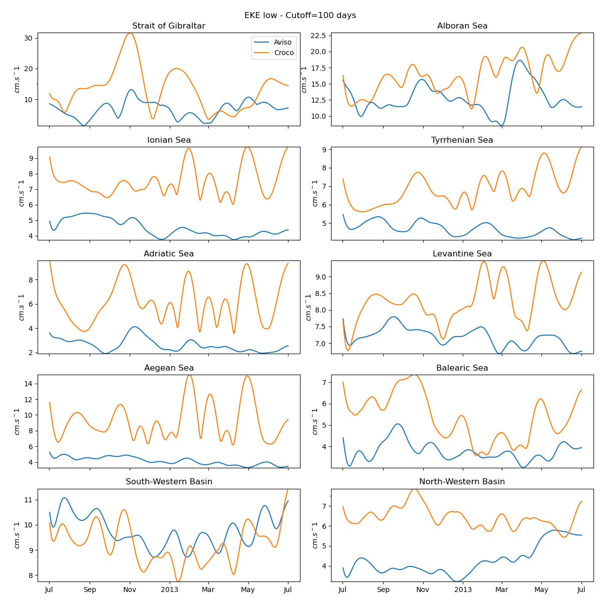
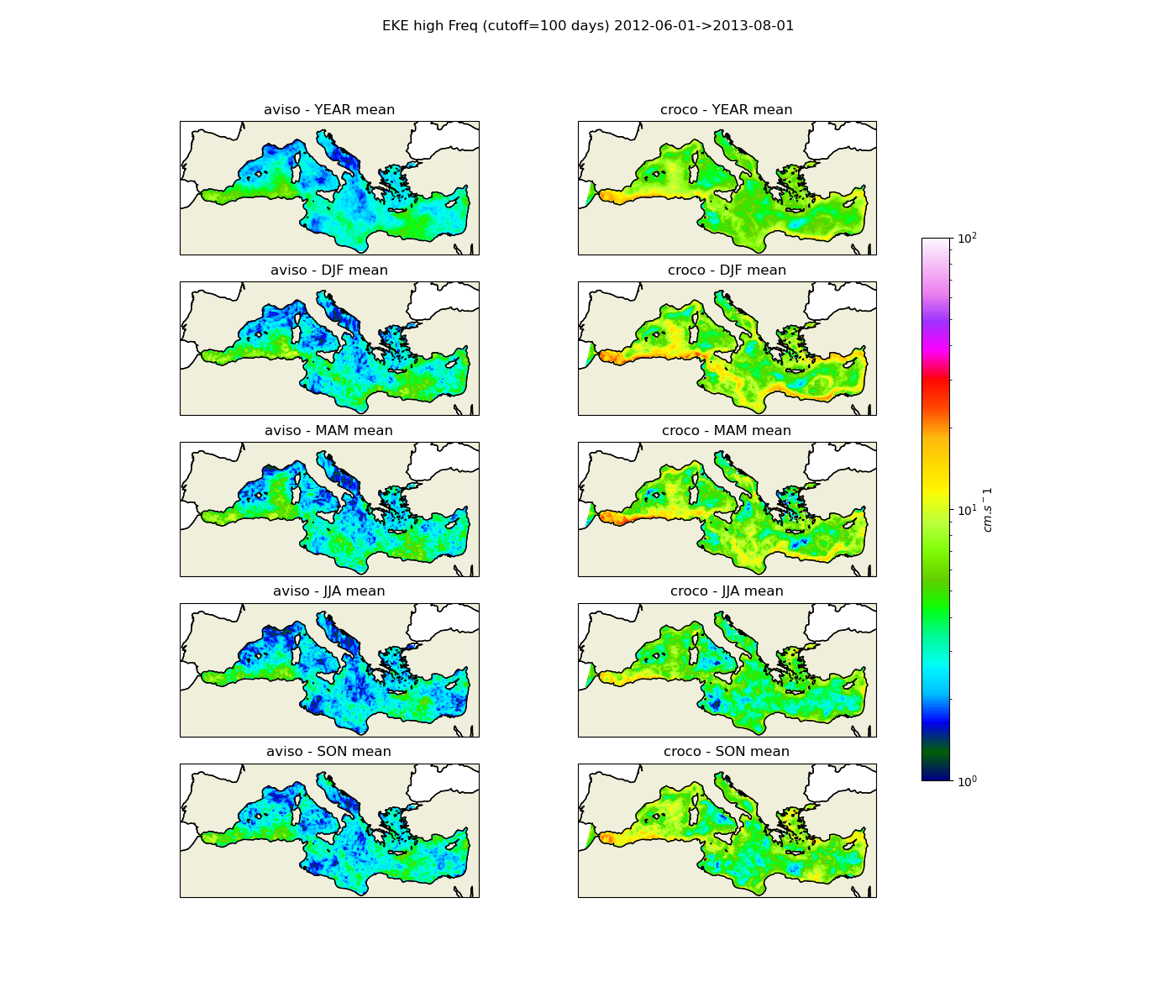
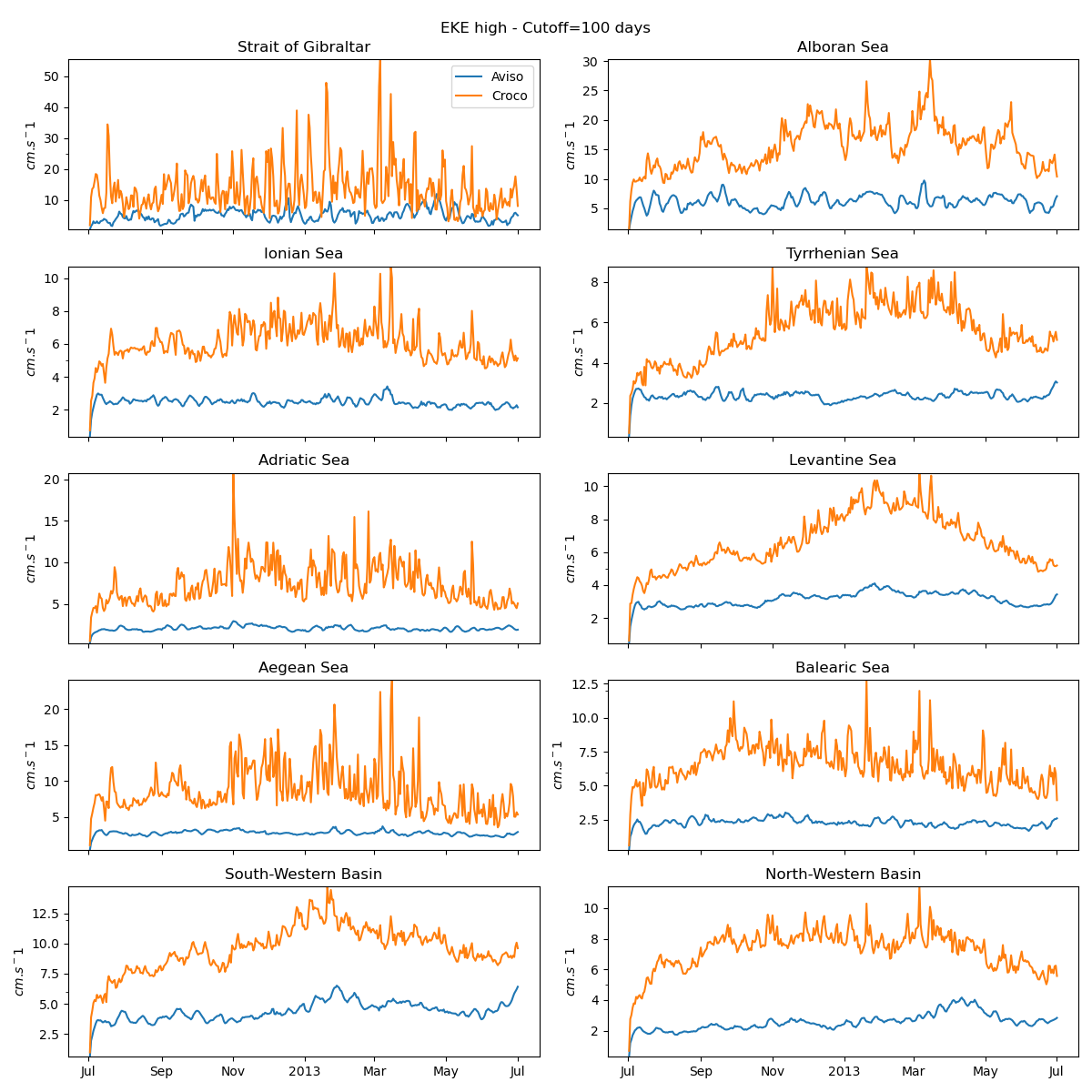
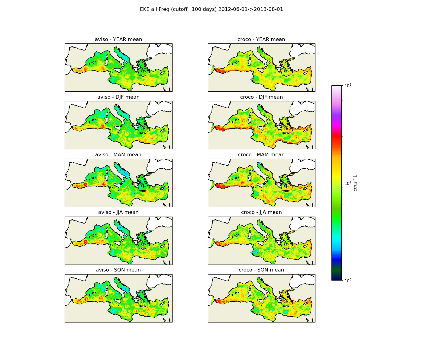
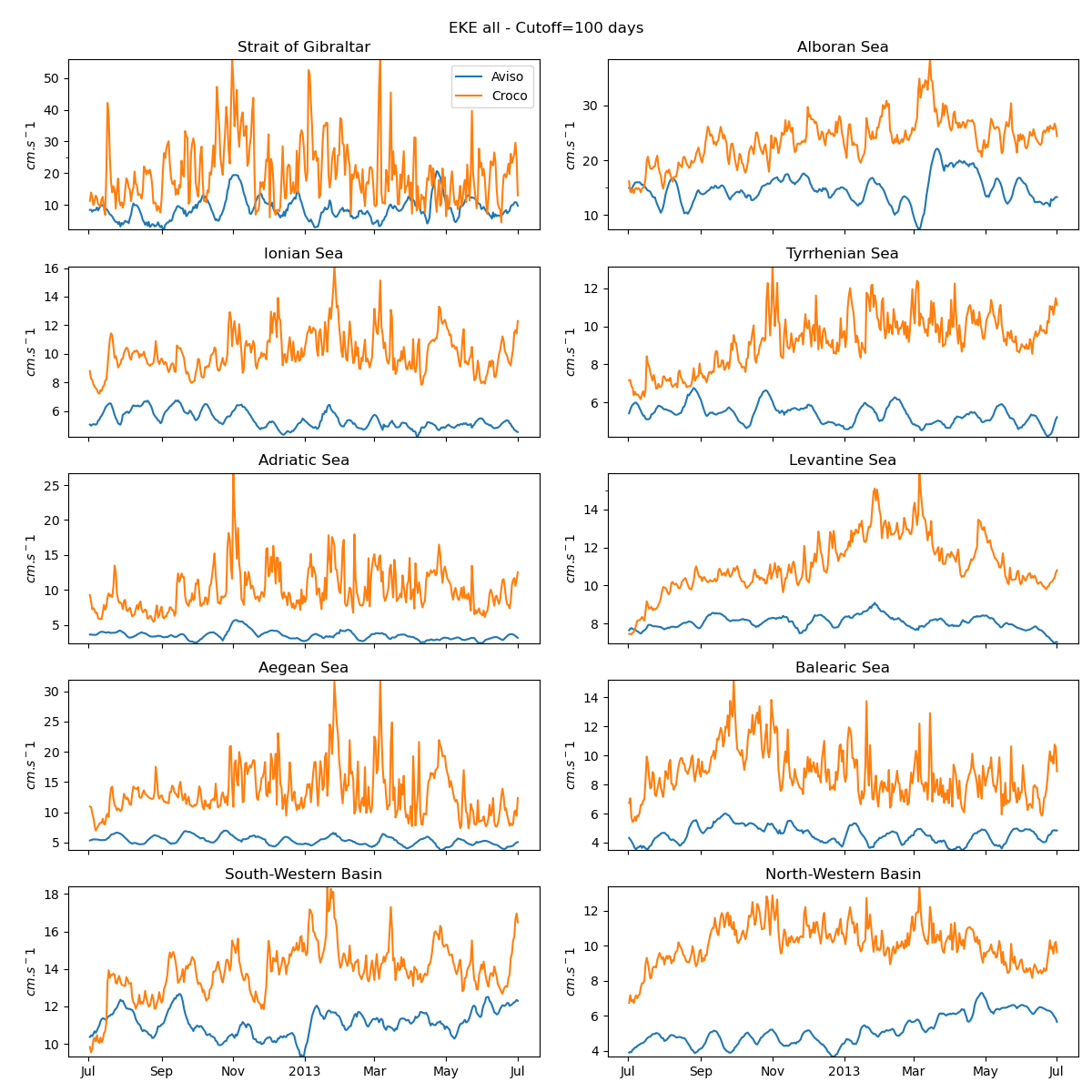
Once the EKE is computed for both Data and model, a temporal filter is applied to separate the low and high components. The filter used is the butterworth filter with a cut-off frequency of 100 days.
What plots ?
Maps of low and high passed EKE comparisons
Spatial mean over the differents basins in mediterranea and plot of the time series
What scripts ?
diags_alti.ipynb is the notebook to use to compute and do the plots